R Basics for Paleoecologists

APD Workshop Series: R Basics for Paleoecologists.

This is meant to be a simple guide to help otherwise busy paleoecologists make use of some helpful tools for conducting research and publishing. All the while, you will also be making your work reproducible.

Required Software and Download Instructions

For this workshop we will be using two separate, but related pieces of open-source software: R and R Studio.

R is a standalone open-source software for statistical analysis. It has an interesting history (you can find more here), but it is both a programming language and an environment within which you can use the language to execute commands. Thus, it is described as the “R Statistical Computing Environment”. R is an instantiation of a tiny universe with many rules, few (or none!) of which you know.

R Studio is a wrapper for R that allows us to see a bit more of what is going on inside of R and to control it through the window rather than exclusively through the “console”. R Studio knows the rules so you don’t have to. Much like a spell-checker in word processing, R Studio checks your code for you. More on this later.

Installing R Statistical Computing Environment

First, you need to install R from cran.r-project.org. Click this link or the logo below, at the top of the page you will find a section titled “Download and Install R” and choose the appropriate download for your operating system (OS).

It should look something like this:

Figure 1. cran.R-project website landing page.

Once you’ve selected the R version for your OS, you’ll be given some download options. Select “base” and download the .exe file (Windows).

Figure 2. cran.R-project windows download options, select ‘base’.

Double-click on this file and follow the instructions from your machine’s prompts for installation. This differs slightly between each operating system and the version of the operating system you’re using.

If you’re using macOS, you will be directed to a slightly different looking page with multiple download options.

Here, you much choose a package based on the version of the macOS you’re using as well as the kind of processor in your machine.

If you’re using macOS 11 or greater (Apple names their updates, so this one is ‘Big Sur’) AND your machine uses an M1 chip, then select the top option (Fig 3:A). If you’re using versions before this (‘High Sierra’) and have an Intel 64-bit chip, then download the second option (Fig 3:B).

Don’t know what kind of chip is in your mac? You can quickly find out by clicking the apple icon at the top right of your screen, then selecting “about this mac”. You should get a window listing the macOS version, kind of machine of you’re using, and details about the processor and memory. Newer macs list the processor as the “Chip”. You can get more detailed instructions for investigating your hardware from Apple’s support page.

Figure 3. cran.R-project macOS download options

For windows users, R will install to your “program files” folder. For macOS users, you will need to move the R.app folder from the package (once opened) and drag it into your applications folder.

Introduction to R Syntax, Objects, and Functions

Second, let’s open up R to make sure that it works and to look at some important features that will help you later on. When you open R, you only get a text window called the console. This is where all of the action happens and as soon as you open R, you’re given some basic, but important information.

Figure 4. R Console with annotations for: A, working directory; B, version; C, citation instructions; and D, the command line.

Note the following: -the working directory is the folder where R looks when it goes to find or write things (Fig. 4:A). -the software version is at the top of the initialization text, this information is important for citations (Fig. 4:B). -the intialization text includes instructions for getting information about licensing, help, and for citing R (Fig. 4:C). -the command line is the line starting with “>”, which is where you politely ask R to do things for you (Fig. 4:D).

We can actually try out a bit of coding at this point. Type the code below in your R console and hit “enter”. You can also copy-paste from this document into the console as well.

citation()

This can also be written as:

citation("base")

Both these commands give us the same result.

## 
## To cite R in publications use:
## 
##   R Core Team (2020). R: A language and environment for statistical
##   computing. R Foundation for Statistical Computing, Vienna, Austria.
##   URL https://www.R-project.org/.
## 
## A BibTeX entry for LaTeX users is
## 
##   @Manual{,
##     title = {R: A Language and Environment for Statistical Computing},
##     author = {{R Core Team}},
##     organization = {R Foundation for Statistical Computing},
##     address = {Vienna, Austria},
##     year = {2020},
##     url = {https://www.R-project.org/},
##   }
## 
## We have invested a lot of time and effort in creating R, please cite it
## when using it for data analysis. See also 'citation("pkgname")' for
## citing R packages.

Congratulations! If this is your first time using R, then you just ran your first function!

Note that “base” gives us the same output because the R Statistical Computing Environment comes with a lot of basic functions (hence “base”) that it can do. Later, we will explore how we can expand R with “packages” written and maintained by other users.

We have accumulated some vocabulary at this point and it is helpful to explain these terms and how they relate to each other here. R will do exactly what you tell it to, so it helps to know how it thinks. The R environment runs almost entirely by creating objects and applying functions to them. Like we experienced above, functions make things happen. In order for R to do things with an object, it has to know that it exists.

We could use “base” above because the citation() is already a part of R and knows where to find it (its always an object). Let’s learn how to create an object.

All coding languages run on syntax (rules for combining things for communication). Here’s some key symbols in R syntax.

Syntax	Action
=	equals sign is used to assign data to objects
<-	arrow-dash is the same as equals sign, assigns data to objects
#	hashes designate non-coding regions, used to annotate code

You can copy-paste the entire section of code below and run it. Another nice thing about R is that you can submit a whole list of commands at once, as long as each of these commands and function are entered correctly. Because my annotations are preceded by a hash “#”, they’re not read as commands. As for whether one should use “=” or “<-”, there are trade-offs to either choice. I use “=” becauese it requires typing fewer characters.

# Here, we use "=" to create an object called "x" and assign it the value of 5.

x = 5

# We can also use "<-" to create another object called "y" and assign it the value of 6.

y <- 6

Once you run the above code, you may notice that basically nothing happened. R happily ran your commands and creates an object named “x” with a value of 5 and an object “y” with a value of 6. You didn’t tell R to give you any output, so none is given. Type “x” in the command line and then hit “enter”. Do the same for “y”. R should return the values each time after you hit “enter”. This is rudimentary, but you are coding now. Also, now that we’ve experienced what R is like, we can gain a better appreciation for what R Studio does for us.

Installing R Studio

Third, you will need to download R Studio and install it. R Studio is available as a “free version” and a “professional” version. The links here go directly to the free version.

The webpage should detect what sort of OS you’re using and suggest the correct version of R Studio. If it does not, there are other download options below which correspond to various OS types and their individual versions. You will notice that the webpage also tells you to install R (which we’ve already done), so you can skip to “2” and download R Studio.

Figure 5. R Studio Download Page.

You’ll get either a .exe or a .pkg file when you download R Studio (depending on OS) and you can then run this file and follow the prompts from the installation wizard. Windows users will find R Studio in their program files while masOS users will have to move the R Studio app into the Applications folder. Make a shortcut to your desktop (Windows) or put the app in your taskbar (macOS) for easy access.

Now, let’s open R Studio and take a look at it. Double-click on the icon.

Figure 6. R Studio window with annotated console pane: A, working directory; B, R version; C, citation info; and D, the command line.

You should have three panes open in the window, as shown in Fig 6. above. The leftmost should look familiar. It is the R console! This is where you’ll enter commands to make R do things. It also shows you some of the same information, such as the location of the working directory (Fig 6:A) and command line (Fig 6:D). You may notice other tabs behind the console titled “Terminal” and “Background jobs”. Stick with the console for now, but this area of the window is dedicated to what R is doing.

On the right, the top pane also has tabs: “Environment” (Fig 6:E), “History” (Fig 6:F), “Connections” (Fig 6:G), and “Tutorial” (Fig 6:G). We will rely on “Environment” and “History” more than the others for this tutorial.

The “Environment” allows us to see inside R’s brain. Let’s take a quick look at how this works by entering the same commands from our first use of base R. You can type these commands manually or copy paste them.

x = 5
y = 6

After you’ve run both commands (after hitting “enter”), you should see the environment update to include the new objects you’ve made. Base R didn’t show you anything, but we demonstrated that R remembered these objects and recalled their values. Here, we can see what R knows.

Figure 7. R Studio showing updated Environment pane after creating objects.

Now click on the “History” tab. Here is where you can find all of the past commands you have given R. This can be helpful for troubleshooting problems. It should look like Figure 8.

Figure 8. Screenshot of R studio window with history tab selected.

The bottom-right pane has several file-navigation related tabs: “Files” (Fig 6:I), “Plots” (Fig 6:J), “Packages” (Fig 6:K), and “Help” (Fig 6:L). There’s other tabs here, but we will make the most use of “Files”, “Plots”, and “Help” during the workshop. “Files” shows you the contents of the working directory as well as the file path to the working directory (below the options - “New Folder”, “Delete”, “Rename”, “More”). This can be really helpful when troubleshooting your code. Remember, R has to be able to find your data. In order to help it do so, you have to know where R thinks it is. R always thinks it is in the working directory and this pane (plus the top of the Console) will help you figure out where R thinks that working directory is.

Another helpful pane in the bottom-right is the “Plots” pane. R Studio saves all of the plots that you make here. Because we’ve already defined two objects, let’s plot them and see what happens.

plot(x, y)

This should create a plot in this pane, looking something like this.

Figure 9. R Studio window showing plot of values of x and y.

Excellent! You’ve already run your first function, defined objects, and then plotted them. This is basically all that R does, but we can create objects with multiple dimensions (vectors, matrices, arrays!) and run complicated functions to evaluate, synthesize, and plot this information.

Setting up R Markdown (Bonus)

At the end of the workshop, we will apply some of our R skills to make an R Markdown document. Markdown is another coding language, but it is native to R Studio and is helpful for presenting results. Let’s set up an R Markdown document and introduce the 4th pane in the R Studio window. At the top right of the R Studio window (not within the panes!) select the “new file” icon (plus sign over a piece of paper) and select the “R Markdown” option.

Figure 10. Screenshot of opening the ‘new file’ option and selecting R Markdown document

You will be prompted to download dependencies for R Markdown. Go ahead and select “yes”.

Figure 11. Screenshot of installation prompt.

R Studio will automatically download and install packages necessary for using R Markdown.

Figure 12. Screenshot of installation progress.

R Markdown will prompt you to give your document a title and to list authors. You can enter any information you want here. Add your name and a provisional title. Make sure the default output is “html”. Outputting to .pdf requires some extra steps (installing LaTex) that can be addressed later. Html output is preferable because it doesn’t have page breaks and it can be printed directly from the web browser.

Figure 13. Screenshot of R Markdown initial screen.

This should open an R markdown document as the fourth pane of the R Studio interface (above the Console). There are a range of document types that you can open, but the ones we will be using are R scripts and R Markdown.

Figure 14. Screenshot of intitial R markdown document.

R Markdown documents open with some information already entered for you. We will discuss more in the workshop on how to make use of these general features, but you can already use the “knit” command to convert this Markdown document to html.

Figure 15. Screenshot of save prompt for R markdown document.

The first time you do this, you’ll have to save the R Markdown (.Rmd) document somewhere. At this point, we are not worrying about file management, so feel free to save it to your “Documents” folder or wherever you prefer.

Figure 16. Screenshot of save option for R markdown document.

You should get output that looks like this. R markdown converts the document’s code into html and outputs the R commands as well as the markdown text. We will use this basic structure to build documents usable for publicatios and project management.

Figure 17. Screenshot of html output from R markdown document.

At last, you have installed and initialized all of the basic tools we will use for the first APD workshop. There are a lot of open-access resources to help you get familiar with R Studio and R Markdown. Please check these out below.

Web Resources

R Studio provides resources for beginners that are free to use.

datacamp also provides some basic instructions for beginners that may be helpful.

James Scott’s Data Science in R: A Gentle Introduction is another good resource that covers much of the same material.

Troubleshooting

Everyone encounters problems along the way and troubleshooting on the web can be helpful. Here’s some suggestions for how to get better search results:

-Include software in search terms “R Studio, installation problems”.
-Include hardware in search terms “R Studio, installation problems, Windows 7”.
-Include names of key websites in search terms “R Studio, installation problems, Windows 7, stack overflow”.
-Include error messages in search terms “R Studio,”error: cannot compile“, Windows 7”.

If you are encountering a problem, it is likely that someone else has also had this issue. Google is useful, but you may find sites like stack overflow to be really useful.

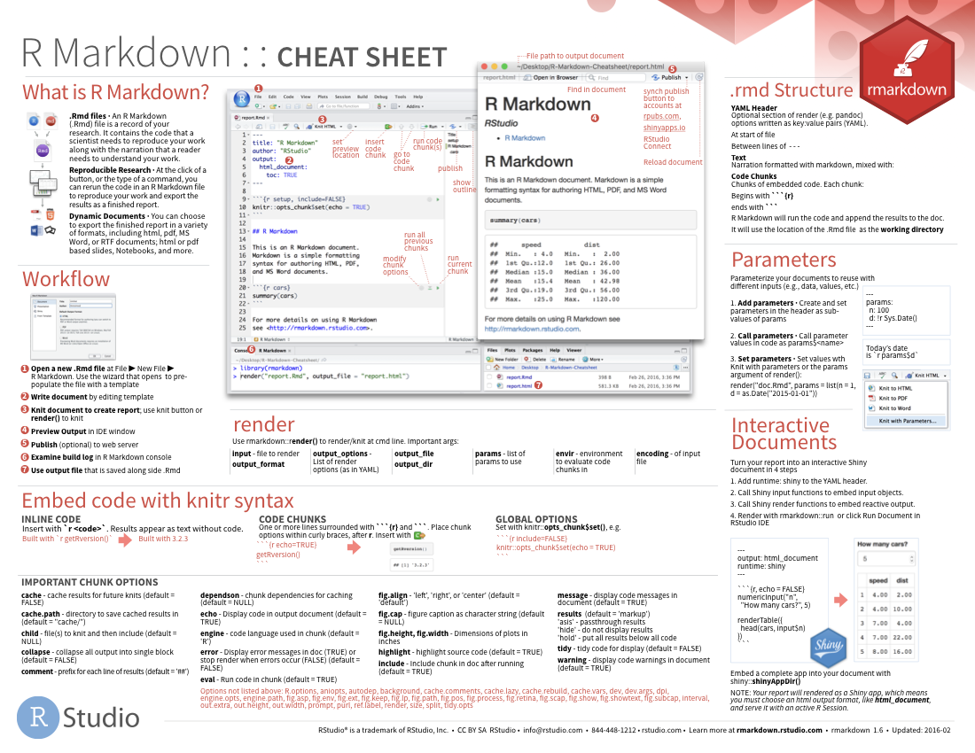
Cheat Sheets

There’s lots of cheat sheets that provide references for syntax, commands, and functions in R Studio and R Markdown. They’re handy and strongly recommended for quick reference.

R Studio cheat sheets

R Markdown cheat sheet